
OMNeT++ simulations can be run under graphical user interfaces like Qtenv that offer visualization and animation in addition to interactive execution and other features. This chapter deals with model visualization.
OMNeT++ essentially provides four main tools for defining and enhancing model visualization:
The following sections will cover the above topics in more detail. But first, let us get acquainted with a new cModule virtual method that one can redefine and place visualization-related code into.
Traditionally, when C++ code was needed to enhance visualization, for example to update a displayed status label or to refresh the position of a mobile node, it was embedded in handleMessage() functions, enclosed in if (ev.isGUI()) blocks. This was less than ideal, because the visualization code would run for all events in that module and not just before display updates when it was actually needed. In Express mode, for example, Qtenv would only refresh the display once every second or so, with a large number of events processed between updates, so visualization code placed inside handleMessage() could potentially waste a significant amount of CPU cycles. Also, visualization code embedded in handleMessage() is not suitable for creating smooth animations.
Starting from OMNeT++ version 5.0, visualization code can be placed into a dedicated method. It is called much more economically, that is, exactly as often as needed.
This method is refreshDisplay(), and is declared on cModule as:
virtual void refreshDisplay() const {}
Components that contain visualization-related code are expected to override refreshDisplay(), and move visualization code such as display string manipulation, canvas figure maintenance and OSG scene graph updates into it.
When and how is refreshDisplay() invoked? Generally, right before the GUI performs a display update. With some additional rules, that boils down to the following:
Here is an example of how one would use it:
void FooModule::refreshDisplay() const
{
    // refresh statistics
    char buf[80];
    sprintf(buf, "Sent:%d  Rcvd:%d", numSent, numReceived);
    getDisplayString()->setTagArg("t", 0, buf);

    // update the mobile node's position
    Point pos = ...  // e.g. invoke a computePosition() method
    getDisplayString()->setTagArg("p", 0, pos.x);
    getDisplayString()->setTagArg("p", 1, pos.y);
}
One useful accessory to refreshDisplay() is the isExpressMode() method of cEnvir. It returns true if the simulation is running under a GUI in Express mode. Visualization code may check this flag and adapt the visualization accordingly. An example:
if (getEnvir()->isExpressMode()) {
    // display throughput statistics
}
else {
    // visualize current frame transmission
}
Overriding refreshDisplay() has several advantages over putting the simulation code into handleMessage(). The first one is clearly performance. When running under Cmdenv, the runtime cost of visualization code is literally zero, and when running in Express mode under Tkenv/Qtenv, it is practically zero because the cost of one update is amortized over several hundred thousand or million events.
The second advantage is also very practical: consistency of the visualization. If the simulation has cross-module dependencies such that an event processed by one module affects the information displayed by another module, with handleMessage()-based visualization the model may have inconsistent visualization until the second module also processes an event and updates its displayed state. With refreshDisplay() this does not happen, because all modules are refreshed together.
The third advantage is separation of concerns. It is generally not a good idea to intermix simulation logic with visualization code, and refreshDisplay() allows one to completely separate the two.
Code in refreshDisplay() should never alter the state of the simulation because that would destroy repeatability, due to the fact that the timing and frequency of refreshDisplay() calls is completely unpredictable from the simulation model's point of view. The fact that the method is declared const gently encourages this behavior.
If visualization code makes use of internal caches or maintains some other mutable state, such data members can be declared mutable to allow refreshDisplay() to change them.
Support for smooth custom animation allows models to visualize their operation using sophisticated animations. The key idea is that the simulation model is called back from the runtime GUI (Qtenv) repeatedly at a reasonable “frame rate,” allowing it to continually update the canvas (2D) and/or the 3D scene to produce fluid animations. Callback means that the refreshDisplay() methods of modules and figures are invoked.
refreshDisplay() knows the animation position from the simulation time and the animation time, a variable also made accessible to the model. If you think about the animation as a movie, animation time is simply the position in seconds in the movie. By default, the movie is played in Qtenv at normal (1x) speed, and then animation time is simply the number of seconds since the start of the movie. The speed control slider in Qtenv's toolbar allows you to play it at higher (2x, 10x, etc.) and lower (0.5x, 0.1x, etc.) speeds; so if you play the movie at 2x speed, animation time will pass twice as fast as real time.
When smooth animation is turned on (more about that later), simulation time progresses in the model (piecewise) linearly. The speed at which the simulation progresses in the movie is called animation speed. Sticking to the movie analogy, when the simulation progresses in the movie 100 times faster than animation time, animation speed is 100.
Certain actions take zero simulation time, but we still want to animate them. Examples of such actions are the sending of a message over a zero-delay link, or a visualized C++ method call between two modules. When these animations play out, simulation is paused and simulation time stays constant until the animation is over. Such periods are called holds.
Smooth animation is a relatively new feature in OMNeT++, and not all simulations need it. Smooth and traditonal, “non-smooth” animation in Qtenv are two distinct modes which operate very differently:
The factor that decides which operation mode is active is the presence of an animation speed. If there is no animation speed, traditional animation is performed; if there is one, smooth animation is done.
The Qtenv GUI has a dialog (Animation Parameters) which displays
the current animation speed, among other things. This dialog allows the
user to check at any time which operation mode is currently active.
Different animation speeds may be appropriate for different animation effects. For example, when animating WiFi traffic where various time slots are on the microsecond scale, an animation speed on the order of 10^-5 might be appropriate; when animating the movement of cars or pedestrians, an animation speed of 1 is a reasonable choice. When several animations requiring different animation speeds occur in the same scene, one solution is to animate the scene using the lowest animation speed so that even the fastest actions can be visually followed by the human viewer.
The solution provided by OMNeT++ for the above problem is the following. Animation speed cannot be controlled explicitly, only requests may be submitted. Several parts of the models may request different animation speeds. The effective animation speed is computed as the minimum of the animation speeds of visible canvases, unless the user interactively overrides it in the UI, for example by imposing a lower or upper limit.
An animation speed requests may be submitted using the setAnimationSpeed()
method of cCanvas.
An example:
cCanvas *canvas = getSystemModule()->getCanvas(); // toplevel canvas
canvas->setAnimationSpeed(2.0, this); // one request
canvas->setAnimationSpeed(1e-6, macModule); // another request
...
canvas->setAnimationSpeed(1.0, this); // overwrite first request
canvas->setAnimationSpeed(0, macModule); // cancel second request
In practice, built-in animation effects such as message sending animation also submit their own animation speed requests internally, so they also affect the effective animation speed chosen by Qtenv.
The current effective animation speed can be obtained from the environment of the simulation (cEnvir, see chapter [18] for context):
double animSpeed = getEnvir()->getAnimationSpeed();
Animation time can be accessed like this:
double animTime = getEnvir()->getAnimationTime();
Animation time starts from zero, and monotonically increases with simulation time and also during “holds”.
As mentioned earlier, a hold interval is an interval when only animation takes place, but simulation time does not progress and no events are processed. Hold intervals are intended for animating actions that take zero simulation time.
A hold can be requested with the holdSimulationFor() method of cCanvas, which accepts an animation time delta as parameter. If a hold request is issued when there is one already in progress, the current hold will be extended as needed to incorporate the request. A hold request cannot be cancelled or shrunk.
cCanvas *canvas = getSystemModule()->getCanvas(); // toplevel canvas
canvas->holdSimulationFor(0.5); // request a 0.5s (animation time) hold
When rendering frames in refreshDisplay()) during a hold, the code can use animation time to determine the position in the animation. If the code needs to know the animation time elapsed since the start of the hold, it should query and remember the animation time when issuing the hold request.
If the code needs to know the animation time remaining until the end of the hold, it can use the getRemainingAnimationHoldTime() method of cEnvir. Note that this is not necessarily the time remaining from its own hold request, because other parts of the simulation might extend the hold.
If a model implements such full-blown animations for a compound module that OMNeT++'s default animations (message sending/method call animations) become a liability, they can be programmatically turned off for that module with cModule's setBuiltinAnimationsAllowed() method:
// disable animations for the toplevel module
cModule *network = getSimulation()->getSystemModule();
network->setBuiltinAnimationsAllowed(false);
Display strings are compact textual descriptions that specify the arrangement and appearance of the graphical representations of modules and connections in graphical user interfaces (currently Tkenv and Qtenv).
Display strings are usually specified in NED's @display property, but it is also possible to modify them programmatically at runtime.
Display strings can be used in the following contexts:
Display strings are specified in @display properties. The property must contain a single string as value. The string should contain a semicolon-separated list of tags. Each tag consists of a key, an equal sign and a comma-separated list of arguments:
@display("p=100,100;b=60,10,rect,blue,black,2")
Tag arguments may be omitted both at the end and inside the parameter list. If an argument is omitted, a sensible default value is used. In the following example, the first and second arguments of the b tag are omitted.
@display("p=100,100;b=,,rect,blue")
Display strings can be placed in the parameters section of module and channel type definitions, and in submodules and connections. The following NED sample illustrates the placement of display strings in the code:
simple Server
{
    parameters:
        @display("i=device/server");
    ...
}

network Example
{
    parameters:
        @display("bgi=maps/europe");
    submodules:
        server: Server {
            @display("p=273,101");
        }
        ...
    connections:
        client1.out --> { @display("ls=red,3"); } --> server.in++;
}
At runtime, every module and channel object has one single display string object, which controls its appearance in various contexts. The initial value of this display string object comes from merging the @display properties occurring at various places in NED files. This section describes the rules for merging @display properties to create the module or channel's display string.
The base NED type's display string is merged into the current display string using the following rules:
The result of merging the @display properties will be used to initialize the display string object (cDisplayString) of the module or channel. The display string object can then still be modified programmatically at runtime.
Example of display string inheritance:
simple Base {
    @display("i=block/queue"); // use a queue icon in all instances
}

simple Derived extends Base {
    @display("i=,red,60");  // ==> "i=block/queue,red,60"
}

network SimpleQueue {
    submodules:
        submod: Derived {
            @display("i=,yellow,-;p=273,101;r=70");
                     // ==> "i=block/queue,yellow;p=273,101;r=70"
        }
        ...
}
The following tags of the module display string are in effect in submodule context, that is, when the module is displayed as a submodule of another module:
The following sections provide an overview and examples for each tag. More detailed information, such as what each tag argument means, is available in Appendix [24].
By default, modules are displayed with a simple default icon, but OMNeT++ comes with a large set of categorized icons that one can choose from. To see what icons are available, look into the images/ folder in the OMNeT++ installation. The stock icons installed with OMNeT++ have several size variants. Most of them have very small (vs), small (s), large (l) and very large (vl) versions.
One can specify the icon with the i tag. The icon name should be given with the name of the subfolder under images/, but without the file name extension. The size may be specified with the icon name suffix (_s for very small, _vl for very large, etc.), or in a separate is tag.
An example that displays the block/source in large size:
@display("i=block/source;is=l");
Icons may also be colorized, which can often be useful. Color can indicate the status or grouping of the module, or simply serve aesthetic purposes. The following example makes the icon 20% red:
@display("i=block/source,red,20")
Modules may also display a small auxiliary icon in the top-right corner of the main icon. This icon can be useful for displaying the status of the module, for example, and can be set with the i2 tag. Icons suitable for use with i2 are in the status/ category.
An example:
@display("i=block/queue;i2=status/busy")

To have a simple but resizable representation for a module, one can use the b tag to create geometric shapes. Currently, oval and rectangle are supported.
The following example displays an oval shape of the size 70x30 with a 4-pixel black border and red fill:
@display("b=70,30,oval,red,black,4")

The p tag allows one to define the position of a submodule or otherwise affect its placement.
The following example will place the module at the given position:
@display("p=50,79");
If the submodule is a module vector, one can also specify in the p tag how to arrange the elements of the vector. They can be arranged in a row, a column, a matrix or a ring. The rest of the arguments in the p tag depend on the layout type:
A matrix layout for a module vector (note that the first two arguments, x and y are omitted, so the submodule matrix as a whole will be placed by the layouter algorithm):
host[20]: Host {
    @display("p=,,m,4,50,50");
}
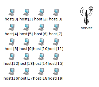
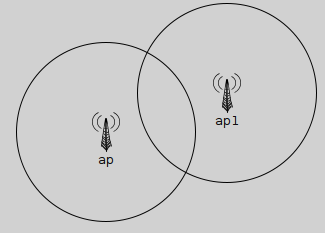
In wireless simulations, it is often useful to be able to display a circle or disc around the module to indicate transmission range, reception range, or interference range. This can be done with the r tag.
In the following example, the module will have a circle with a 90-unit radius around it as a range indicator:
submodules:
    ap: AccessPoint {
        @display("p=50,79;r=90");
    }
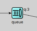
If a module contains a queue object (cQueue), it is possible to let the graphical user interface display the queue length next to the module icon. To achieve that, one needs to specify the queue object's name (the string set via the setName() method) in the q display string tag. OMNeT++ finds the queue object by traversing the object tree inside the module.
The following example displays the length of the queue named "jobQueue":
@display("q=jobQueue");
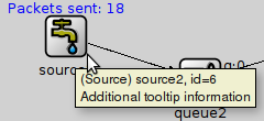
It is possible to have a short text displayed next to or above the module icon or shape using the t tag. The tag lets one specify the placement (left, right, above) and the color of the text. To display text in a tooltip, use the tt tag.
The following example displays text above the module icon, and also adds tooltip text that can be seen by hovering over the module icon with the mouse.
@display("t=Packets sent: 18;tt=Additional tooltip information");
For a detailed descripton of the display string tags, check Appendix [24].
The following tags of the module display string are in effect when the module itself is opened in a GUI. These tags mostly deal with the visual properties of the background rectangle.
In the following example, the background area is defined to be 6000x4500 units, and the map of Europe is used as a background, stretched to fill the whole area. A grid is also drawn, with 1000 units between major ticks, and 2 minor ticks per major tick.
network EuropePlayground
{
    @display("bgb=6000,4500;bgi=maps/europe,s;bgg=1000,2,grey95;bgu=km");
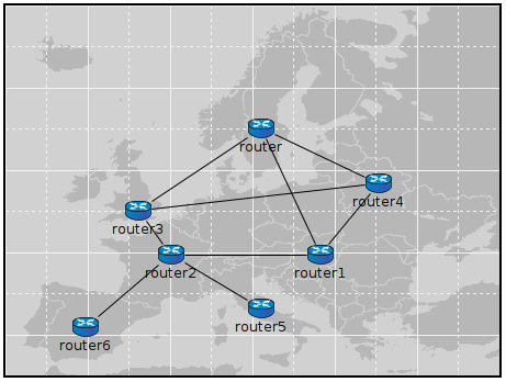
The bgu tag deserves special attention. It does not affect the visual appearance, but instead it is a hint for model code on how to interpret coordinates and distances in this compound module. The above example specifies bgu=km, which means that if the model attaches physical meaning to coordinates and distances, then those numbers should be interpreted as kilometers.
More detailed information, such as what each tag argument means, is available in Appendix [24].
Connections may also have display strings. Connections inherit the display string property from their channel types, in the same way as submodules inherit theirs from module types. The default display strings are empty.
Connections support the following tags:
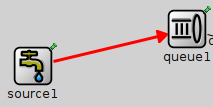
Example of a thick, red connection:
source1.out --> { @display("ls=red,3"); } --> queue1.in++;
More detailed information, such as what each tag argument means, is available in Appendix [24].
Message display strings affect how messages are shown during animation. By default, they are displayed as a small filled circle, in one of 8 basic colors (the color is determined as message kind modulo 8), and with the message class and/or name displayed under it. The latter is configurable in the Options dialog of Tkenv and Qtenv, and message kind dependent coloring can also be turned off there.
Message objects do not store a display string by default. Instead, cMessage defines a virtual getDisplayString() method that one can override in subclasses to return an arbitrary string. The following example adds a display string to a new message class:
class Job : public cMessage
{
  public:
    const char *getDisplayString() const {return "i=msg/packet;is=vs";}
    //...
};
Since message classes are often defined in msg files (see chapter [6]), it is often convenient to let the message compiler generate the getDisplayString() method. To achieve that, add a string field named displayString with an initializer to the message definition. The message compiler will generate setDisplayString() and getDisplayString() methods into the new class, and also set the initial value in the constructor.
An example message file:
message Job
{
    string displayString = "i=msg/package_s,kind";
    //...
}
The following tags can be used in message display strings:
The following example displays a small red box icon:
@display("i=msg/box,red;is=s");
The next one displays a 15x15 rectangle, with while fill, and with a border color dependent on the message kind:
@display("b=15,15,rect,white,kind,5");
More detailed information, such as what each tag argument means, is available in Appendix [24].
Parameters of the module or channel containing the display string can be substituted into the display string with the $parameterName notation:
Example:
simple MobileNode
{
    parameters:
        double xpos;
        double ypos;
        string fillColor;
        // get the values from the module parameters xpos,ypos,fillcolor
        @display("p=$xpos,$ypos;b=60,10,rect,$fillColor,black,2");
}
A color may be given in several forms. One is English names: blue, lightgrey, wheat, etc.; the list includes all standard SVG color names.
Another acceptable form is the HTML RGB syntax: #rgb or #rrggbb, where r,g,b are hex digits.
It is also possible to specify colors in HSB (hue-saturation-brightness) as @hhssbb (with h, s, b being hex digits). HSB makes it easier to scale colors e.g. from white to bright red.
One can produce a transparent background by specifying a hyphen ("-") as background color.
In message display strings, kind can also be used as a special color name. It will map message kind to a color. (See the getKind() method of cMessage.)
The "i=" display string tag allows for colorization of icons. It accepts a target color and a percentage as the degree of colorization. Percentage has no effect if the target color is missing. Brightness of the icon is also affected -- to keep the original brightness, specify a color with about 50% brightness (e.g. #808080 mid-grey, #008000 mid-green).
Examples:
Colorization works with both submodule and message icons.
In the current OMNeT++ version, module icons are PNG or GIF files. The icons shipped with OMNeT++ are in the images/ subdirectory. The IDE, Tkenv and Qtenv all need the exact location of this directory to be able to load the icons.
Icons are loaded from all directories in the image path, a semicolon-separated list of directories. The default image path is compiled into Tkenv and Qtenv with the value "<omnetpp>/images;./images". This works fine (unless the OMNeT++ installation is moved), and the ./images part also allows icons to be loaded from the images/ subdirectory of the current directory. As users typically run simulation models from the model's directory, this practically means that custom icons placed in the images/ subdirectory of the model's directory are automatically loaded.
The compiled-in image path can be overridden with the OMNETPP_IMAGE_PATH environment variable. The way of setting environment variables is system specific: in Unix, if one is using the bash shell, adding a line
export OMNETPP_IMAGE_PATH="$HOME/omnetpp/images;./images"
to ~/.bashrc or ~/.bash_profile will do; on Windows, environment variables can be set via the My Computer --> Properties dialog.
One can extend the image path from omnetpp.ini with the image-path option, which is prepended to the environment variable's value.
[General]
image-path = "/home/you/model-framework/images;/home/you/extra-images"
Icons are organized into several categories, represented by folders. These categories include:
Icon names to be used with the i, bgi and other tags should contain the subfolder (category) name but not the file extension. For example, /opt/omnetpp/images/block/sink.png should be referred to as block/sink.
Icons come in various sizes: normal, large, small, very small, very large. Sizes are encoded into the icon name's suffix: _vl, _l, _s, _vs. In display strings, one can either use the suffix ("i=device/router_l"), or the "is" (icon size) display string tag ("i=device/router;is=l"), but not both at the same time (we recommend using the is tag.)
OMNeT++ implements an automatic layouting feature, using a variation of the Spring Embedder algorithm. Modules which have not been assigned explicit positions via the "p=" tag will be automatically placed by the algorithm.
Spring Embedder is a graph layouting algorithm based on a physical model. Graph nodes (modules) repel each other like electric charges of the same sign, and connections act as springs that pull nodes together. There is also friction built in, in order to prevent oscillation of the nodes. The layouting algorithm simulates this physical system until it reaches equilibrium (or times out). The physical rules above have been slightly tweaked to achieve better results.
The algorithm doesn't move any module which has fixed coordinates. Modules that are part of a predefined arrangement (row, matrix, ring, etc., defined via the 3rd and further args of the "p=" tag) will be moved together, to preserve their relative positions.
Caveats:
It is often useful to manipulate the display string at runtime. Changing colors, icon, or text may convey status change, and changing a module's position is useful when simulating mobile networks.
Display strings are stored in cDisplayString objects inside channels, modules and gates. cDisplayString also lets one manipulate the string.
As far as cDisplayString is concerned, a display string (e.g. "p=100,125;i=cloud") is a string that consist of several tags separated by semicolons, and each tag has a name and after an equal sign, zero or more arguments separated by commas.
The class facilitates tasks such as finding out what tags a display string has, adding new tags, adding arguments to existing tags, removing tags or replacing arguments. The internal storage method allows very fast operation; it will generally be faster than direct string manipulation. The class doesn't try to interpret the display string in any way, nor does it know the meaning of the different tags; it merely parses the string as data elements separated by semicolons, equal signs and commas.
To get a pointer to a cDisplayString object, one can call the components's getDisplayString() method.
The display string can be overwritten using the parse() method. Tag arguments can be set with setTagArg(), and tags removed with removeTag().
The following example sets a module's position, icon and status icon in one step:
cDisplayString& dispStr = getDisplayString();
dispStr.parse("p=40,20;i=device/cellphone;i2=status/disconnect");
Setting an outgoing connection's color to red:
cDisplayString& connDispStr = gate("out")->getDisplayString();
connDispStr.parse("ls=red");
Setting module background and grid with background display string tags:
cDisplayString& parentDispStr = getParentModule()->getDisplayString();
parentDispStr.parse("bgi=maps/europe;bgg=100,2");
The following example updates a display string so that it contains the p=40,20 and i=device/cellphone tags:
dispStr.setTagArg("p", 0, 40);
dispStr.setTagArg("p", 1, 20);
dispStr.setTagArg("i", 0, "device/cellphone");
Modules can display a transient bubble with a short message (e.g. "Going down" or "Connection estalished") by calling the bubble() method of cComponent. The method takes the string to be displayed as a const char * pointer.
An example:
bubble("Going down!");
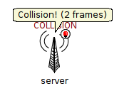
If the module often displays bubbles, it is recommended to make the corresponding code conditional on hasGUI(). The hasGUI() method returns false if the simulation is running under Cmdenv.
if (hasGUI()) {
    char text[32];
    sprintf(text, "Collision! (%s frames)", numCollidingFrames);
    bubble(text);
}
The canvas is the 2D drawing API of OMNeT++. Using the canvas, one can display lines, curves, polygons, images, text items and their combinations, using colors, transparency, geometric transformations, antialiasing and more. Drawings created with the canvas API can be viewed when the simulation is run under a graphical user interface (Tkenv or Qtenv).
Use cases for the canvas API include displaying textual annotations, status information, live statistics in the form of plots, charts, gauges, counters, etc. Other types of simulations may call for different types of graphical presentation. For example, in mobile and wireless simulations, the canvas API can be used to draw the scene including a background (like a street map or floor plan), mobile objects (vehicles, people), obstacles (trees, buildings, hills), antennas with orientation, and also extra information like connectivity graph, movement trails, individual transmissions and so on.
An arbitrary number of drawings (canvases) can be created, and every module already has one by default. A module's default canvas is the one on which the module's submodules and internal connections are also displayed, so the canvas API can be used to enrich the default, display string based presentation of a compound module.
OMNeT++ calls the items that appear on a canvas figures. The corresponding C++ types are cCanvas and cFigure. In fact, cFigure is an abstract base class, and different kinds of figures are represented by various subclasses of cFigure.
Figures can be declared statically in NED files using @figure properties, and can also be accessed, created and manipulated programmatically at runtime.
A canvas is represented by the cCanvas C++ class. A module's default canvas can be accessed with the getCanvas() method of cModule. For example, a toplevel submodule can get hold of the network's canvas with the following line:
cCanvas *canvas = getParentModule()->getCanvas();
Using the canvas pointer, it is possible to check what figures it contains, add new figures, manipulate existing ones, and so on.
New canvases can be created by simply creating new cCanvas objects, like so:
cCanvas *canvas = new cCanvas("liveStatistics"); // arbitrary name string
To view the contents of these additional canvases in Tkenv or Qtenv, one needs to navigate to the canvas' owner object (which will usually be the module that created the canvas), view the list of objects it contains, and double-click the canvas in the list. Giving meaningful names to extra canvas objects like in the example above can simplify the process of locating them in the Tkenv/Qtenv GUI.
The base class of all figure classes is cFigure. The class hierarchy is shown in figure below.

In subsequent sections, we'll first describe features that are common to all figures, then we'll briefly cover each figure class. Finally, we'll look into how one can define new figure types.
Figures on a canvas are organized into a tree. The canvas has a (hidden) root figure, and all toplevel figures are children of the root figure. Any figure may contain child figures, not only dedicated ones like cGroupFigure.
Every figure also has a name string, inherited from cNamedObject. Since figures are in a tree, every figure also has a hierarchical name. It consists of the names of figures in the path from the root figure down to the the figure, joined with dots. (The name of the root figure itself is omitted.)
Child figures can be added to a figure with the addFigure() method, or inserted into the child list of a figure relative to a sibling with the insertBefore() / insertAfter() methods. addFigure() has two flavours: one for appending, and one for inserting at a numeric position. Child figures can be accessed by name (getFigure(name)), or enumerated by index in the child list (getFigure(k), getNumFigures()). One can obtain the index of a child figure using findFigure(). The removeFromParent() method can be used to remove a figure from its parent.
For convenience, cCanvas also has addFigure(), getFigure(), getNumFigures() and other methods for managing toplevel figures without the need to go via the root figure.
The following code enumerates the children of a figure named "group1":
cFigure *parent = canvas->getFigure("group1");
ASSERT(parent != nullptr);
for (int i = 0; i < parent->getNumFigures(); i++)
    EV << parent->getFigure(i)->getName() << endl;
It is also possible to locate a figure by its hierarchical name (getFigureByPath()), and to find figure by its (non-hierarchical) name anywhere in a figure subtree (findFigureRecursively()).
The dup() method of figure classes only duplicates the very figure on which it was called. (The duplicate will not have ay children.) To clone a figure including children, use the dupTree() method.
As mentioned earlier, figures can be defined in the NED file, so they don't always need to be created programmatically. This possibility is useful for creating static backgrounds or statically defining placeholders for dinamically displayed items, among others. Figures defined from NED can be accessed and manipulated from C++ code in the same way as dynamically created ones.
Figures are defined in NED by adding @figure properties to a module definition. The hierarchical name of the figure goes into the property index, that is, in square brackets right after @figure. The parent of the figure must already exist, that is, when defining foo.bar.baz, both foo and foo.bar must have already been defined (in NED).
Type and various attributes of the figure go into property body, as key-valuelist pairs. type=line creates a cLineFigure, type=rectangle creates a cRectangleFigure, type=text creates a cTextFigure, and so on; the list of accepted types is given in appendix [25]. Further attributes largely correspond to getters and setters of the C++ class denoted by the type attribute.
The following example creates a green rectangle and the text "placeholder" in it in NED, and the subsequent C++ code changes the same text to "Hello World!".
NED part:
module Foo
{
    @display("bgb=800,500");
    @figure[box](type=rectangle; coords=10,50; size=200,100; fillColor=green);
    @figure[box.label](type=text; coords=20,80; text=placeholder);
}
And the C++ part:
// we assume this code runs in a submodule of the above "Foo" module
cCanvas *canvas = getParentModule()->getCanvas();

// obtain the figure pointer by hierarchical name, and change the text:
cFigure *figure = canvas->getFigureByPath("box.label")
cTextFigure *textFigure = check_and_cast<cTextFigure *>(figure);
textFigure->setText("Hello World!");
The stacking order (a.k.a. Z-order) of figures is jointly determined by the child order and the cFigure attribute called Z-index, with the latter taking priority. Z-index is not used directly, but an effective Z-index is computed instead, as the sum of the Z-index values of the figure and all its ancestors up to the root figure.
A figure with a larger effective Z-index will be displayed above figures with smaller effective Z-indices, regardless of their positions in the figure tree. Among figures whose effective Z-indices are equal, child order determines the stacking order. If two such figures are siblings, the one that occurs later in the child list will be drawn above the other. For figures that are not siblings, the child order within the first common ancestor matters. There are several methods for managing stacking order: setZIndex(), getZIndex(), getEffectiveZIndex(), insertAbove(), insertBelow(), isAbove(), isBelow(), raiseAbove(), lowerBelow(), raiseToTop(), lowerToBottom().
One of the most powerful features of the Canvas API is being able to assign geometric transformations to figures. OMNeT++ uses 2D homogeneous transformation matrices, which are able to express affine transforms such as translation, scaling, rotation and skew (shearing). The transformation matrix used by OMNeT++ has the following format:
| a | c | t1 |
| b | d | t2 |
| 0 | 0 | 1 |
In a nutshell, given a point with its (x, y) coodinates, one can obtain the transformed version of it by multiplying the transformation matrix by the (x \ y \ 1) column vector (a.k.a. homogeneous coordinates), and dropping the third component:
| x' |
| y' |
| 1 |
| a | c | t1 |
| b | d | t2 |
| 0 | 0 | 1 |
| x |
| y |
| 1 |
The result is the point (ax+cy+t1, bx+dy+t2). As one can deduce, a, b, c, d are responsible for rotation, scaling and skew, and t1 and t2 for translation. Also, transforming a point by matrix T1 and then by T2 is equivalent to transforming the point by the matrix T2 T1 due to the associativity of matrix multiplication.
Transformation matrices are represented in OMNeT++ by the cFigure::Transform class.
A cFigure::Transform transformation matrix can be initialized in several ways. First, it is possible to assign its a, b, c, d, t1, t2 members directly (they are public), or via a six-argument constructor. However, it is usually more convenient to start from the identity transform (as created by the default constructor), and invoke one or more of its several scale(), rotate(), skewx(), skewy() and translate() member functions. They update the matrix to (also) perform the given operation (scaling, rotation, skewing or translation), as if left-multiplied by a temporary matrix that corresponds to the operation.
The multiply() method allows one to combine transformations: t1.multiply(t2) sets t1 to the product t2*t1.
To transform a point (represented by the class cFigure::Point), one can use the applyTo() method of Transform. The following code fragment should clarify this:
// allow Transform and Point to be referenced without the cFigure:: prefix
typedef cFigure::Transform Transform;
typedef cFigure::Point Point;

// create a matrix that scales by 2, rotates by 45 degrees, and translates by (100,0)
Transform t = Transform().scale(2.0).rotate(M_PI/4).translate(100,0);

// apply the transform to the point (10, 20)
Point p(10, 20);
Point p2 = t.applyTo(p);
Every figure has an associated transformation matrix, which affects how the figure and its figure subtree are displayed. In other words, the way a figure displayed is affected by its own transformation matrix and the transformation matrices of all of its ancestors, up to the root figure of the canvas. The effective transform will be the product of those transformation matrices.
A figure's transformation matrix is directly accessible via cFigure's getTransform(), setTransform() member functions. For convenience, cFigure also has several scale(), rotate(), skewx(), skewy() and translate() member functions, which directly operate on the internal transformation matrix.
Some figures have visual aspects that are not, or only optionally affected by the transform. For example, the size and orientation of the text displayed by cLabelFigure, in contrast to that of cTextFigure, is unaffected by transforms (and of manual zoom as well). Only the position is transformed.
In addition to the translate(), scale(), rotate(), etc. functions that update the figure's transformation matrix, figures also have a move() method. move(), like translate(), also moves the figure by a dx, dy offset. However, move() works by changing the figure's coordinates, and not by changing the transformation matrix.
Since every figure class stores and interprets its position differently, move() is defined for each figure class independently. For example, cPolylineFigure's move() changes the coordinates of each point.
move() is recursive, that is, it not only moves the figure on which it was called, but also its children. There is also a non-recursive variant, called moveLocal().
Figures have a visibility flag that controls whether the figure is displayed. Hiding a figure via the flag will hide the whole figure subtree, not just the figure itself. The flag can be accessed via the isVisible(), setVisible() member functions of cFigure.
Figures can also be assigned a number of textual tags. Tags do not directly affect rendering, but graphical user interfaces that display canvas content, namely Tkenv and Qtenv, offer functionality to interactively show/hide figures based on tags they contain. This GUI figure filter allows one to express conditions like "Show only figures that have tag foo or bar, but among them, hide those that also contain tag baz". Tag-based filtering and the visibility flag are in AND relationship -- figures hidden via setVisible(false) cannot be displayed using tags. Also when a figure is hidden using the tag filter, its figure subtree will also be hidden.
The tag list of a figure can be accessed with the getTags() and setTags() cFigure methods. They return/accept a single string that contains the tags separated by spaces (a tag itself cannot contain a space.)
Tags functionality, when used carefully, allows one to define "layers" that can be turned on/off from Tkenv/Qtenv.
Figures may be assigned a tooltip text using the setTooltip() method. The tooltip is shown in the runtime GUI when one hovers with the mouse over the figure.
In the visualization of many simulations, some figures correspond to certain objects in the simulation model. For example, a truck image may correspond to a module that represents the mobile node in the simulation. Or, an inflating disc that represents a wireless signal may correspond to a message (cMessage) in the simulation.
One can set the associated object on a figure using the setAssociatedObject() method. The GUI can use this information provide a shortcut access to the associated object, for example select the object in an inspector when the user clicks the figure, or display the object's tooltip over the figure if it does not have its own.
Points are represented by the cFigure::Point struct:
struct Point {
    double x, y;
    ...
};
In addition to the public x, y members and a two-argument constructor for convenient initialization, the struct provides overloaded operators (+,-,*,/) and some utility functions like translate(), distanceTo() and str().
Rectangles are represented by the cFigure::Rectangle struct:
struct Rectangle {
    double x, y,
    double width, height;
    ...
};
A rectangle is specified with the coordinates of their top-left corner, their width and height. The latter two are expected to be nonnegative. In addition to the public x, y, width, height members and a four-argument constructor for convenient initialization, the struct also has utility functions like getCenter(), getSize(), translate() and str().
Colors are represented by the cFigure::Color struct as 24-bit RGB colors:
struct Color {
    uint8_t red, green, blue;
    ...
};
In addition to the public red, green, blue members and a three-argument constructor for convenient initialization, the struct also has a string-based constructor and str() function. The string form accepts various notations: HTML colors (#rrggbb), HSB colors in a similar notation (@hhssbb), and English color names (SVG and X11 color names, to be more precise.)
However, one doesn't need to use Color directly. There are also predefined constants for the basic colors (BLACK, WHITE, GREY, RED, GREEN, BLUE, YELLOW, CYAN, MAGENTA), as well as a collection of carefully chosen dark and light colors, suitable for e.g. chart drawing, in the arrays GOOD_DARK_COLORS[] and GOOD_LIGHT_COLORS[]; for convenience, the number of colors in each are in the NUM_GOOD_DARK_COLORS and NUM_GOOD_LIGHT_COLORS constants).
The following ways of specifying colors are all valid:
cFigure::BLACK;
cFigure::Color("steelblue");
cFigure::Color("#3d7a8f");
cFigure::Color("@20ff80");
cFigure::GOOD_DARK_COLORS[2];
cFigure::GOOD_LIGHT_COLORS[intrand(NUM_GOOD_LIGHT_COLORS)];
The requested font for text figures is represented by the cFigure::Font struct. It stores the typeface, font style and font size in one.
struct Font {
    std::string typeface;
    int pointSize;
    uint8_t style;
    ...
};
The font does not need to be fully specified, there are some defaults. When typeface is set to the empty string or when pointSize is zero or a negative value, that means that the default font or the default size should be used, respectively.
The style field can be either FONT_NONE, or the binary OR of the following constants: FONT_BOLD, FONT_ITALIC, FONT_UNDERLINE.
The struct also has a three-argument constructor for convenient initialization, and an str() function that returns a human-readable text representation of the contents.
Some examples:
cFigure::Font("Arial");  // default size, normal
cFigure::Font("Arial", 12);  // 12pt, normal
cFigure::Font("Arial", 12, cFigure::FONT_BOLD | cFigure::FONT_ITALIC);
cFigure also contains a number of enums as inner types to describe various line, shape, text and image properties. Here they are:
LineStyle
Values: LINE_SOLID, LINE_DOTTED, LINE_DASHED
This enum (cFigure::LineStyle) is used by line and shape figures to determine their line/border style. The precise graphical interpretation, e.g. dash lengths for the dashed style, depends on the graphics library that the GUI was implemented with.
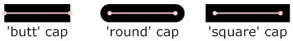
CapStyle
Values: CAP_BUTT, CAP_ROUND, CAP_SQUARE
This enum is used by line and path figures, and it indicates the shape to be used at the end of the lines or open subpaths.
JoinStyle
Values: JOIN_BEVEL, JOIN_ROUND, JOIN_MITER
This enum indicates the shape to be used when two line segments are joined, in line or shape figures.

FillRule
Values: FILL_EVENODD, FILL_NONZERO.
This enum determines which regions of a self-intersecting shape should be considered to be inside the shape, and thus be filled.

Arrowhead
Values: ARROW_NONE, ARROW_SIMPLE, ARROW_TRIANGLE, ARROW_BARBED.
Some figures support displaying arrowheads at one or both ends of a line. This enum determines the style of the arrowhead to be used.

Interpolation
Values: INTERPOLATION_NONE, INTERPOLATION_FAST, INTERPOLATION_BEST.
Interpolation is used for rendering an image when it is not displayed at its native resolution. This enum indicates the algorithm to be used for interpolation.
The mode none selects the "nearest neighbor" algorithm. Fast emphasizes speed, and best emphasizes quality; however, the exact choice of algorithm (bilinear, bicubic, quadratic, etc.) depends on features of the graphics library that the GUI was implemented with.
Anchor
Values:
ANCHOR_CENTER, ANCHOR_N, ANCHOR_E, ANCHOR_S, ANCHOR_W,
ANCHOR_NW, ANCHOR_NE, ANCHOR_SE, ANCHOR_SW;
ANCHOR_BASELINE_START, ANCHOR_BASELINE_MIDDLE,
ANCHOR_BASELINE_END.
Some figures like text and image figures are placed by specifying a single point (position) plus an anchor mode, a value from this enum. The anchor mode indicates which point of the bounding box of the figure should be positioned over the specified point. For example, when using ANCHOR_N, the figure is placed so that its top-middle point falls at the specified point.
The last three, baseline constants are only used with text figures, and indicate that the start, middle or end of the text's baseline is the anchor point.
Now that we know all about figures in general, we can look into the specific figure classes provided by OMNeT++.
cAbstractLineFigure is the common base class for various line figures, providing line color, style, width, opacity, arrowhead and other properties for them.
Line color can be set with setLineColor(), and line width with setLineWidth(). Lines can be solid, dashed, dotted, etc.; line style can be set with setLineStyle(). The default line color is black.
Lines can be partially transparent. This property can be controlled with setLineOpacity() that takes a double between 0 and 1: a zero argument means fully transparent, and one means fully opaque.
Lines can have various cap styles: butt, square, round, etc., which can be selected with setCapStyle(). Join style, which is a related property, is not part of cAbstractLineFigure but instead added to specific subclasses where it makes sense.
Lines may also be augmented with arrowheads at either or both ends. Arrowheads can be selected with setStartArrowhead() and setEndArrowhead().
Transformations such as scaling or skew do affect the width of the line as it is rendered on the canvas. Whether zooming (by the user) should also affect it can be controlled by setting a flag (setZoomLineWidth()). The default is non-zooming lines.
Specifying zero for line width is currently not allowed. To hide the line,
use setVisible(false).
cLineFigure displays a single straight line segment. The endpoints of the line can be set with the setStart()/setEnd() methods. Other properties such as color and line style are inherited from cAbstractLineFigure.
An example that draws an arrow from (0,0) to (100,100):
cLineFigure *line = new cLineFigure("line");
line->setStart(cFigure::Point(0,0));
line->setEnd(cFigure::Point(100,50));
line->setLineWidth(2);
line->setEndArrowhead(cFigure::ARROW_BARBED);
The result:

cArcFigure displays an axis-aligned arc. (To display a non-axis-aligned arc, apply a transform to cArcFigure, or use cPathFigure.) The arc's geometry is determined by the bounding box of the circle or ellipse, and a start and end angle; they can be set with the setBounds(), setStartAngle() and setEndAngle() methods. Other properties such as color and line style are inherited from cAbstractLineFigure.
For angles, zero points east. Angles that go counterclockwise are positive, and those that go clockwise are negative.
Here is an example that draws a blue arc with an arrowhead that goes counter-clockwise from 3 hours to 12 hours on the clock:
cArcFigure *arc = new cArcFigure("arc");
arc->setBounds(cFigure::Rectangle(10,10,100,100));
arc->setStartAngle(0);
arc->setEndAngle(M_PI/2);
arc->setLineColor(cFigure::BLUE);
arc->setEndArrowhead(cFigure::ARROW_BARBED);
The result:

By default, cPolylineFigure displays multiple connecting straight line segments. The class stores geometry information as a sequence of points. The line may be smoothed, so the figure can also display complex curves.
The points can be set with setPoints() that takes std::vector<Point>, or added one-by-one using addPoint(). Elements in the point list can be read and overwritten (getPoint(), setPoint()). One can also insert and remove points (insertPoint() and removePoint().
A smoothed line is drawn as a series of Bezier curves, which touch the start point of the first line segment, the end point of the last line segment, and the midpoints of intermediate line segments, while intermediate points serve as control points. Smoothing can be turned on/off using setSmooth().
Additional properties such as color and line style are inherited from cAbstractLineFigure. Line join style (which is not part of cAbstractLineFigure) can be set with setJoinStyle().
Here is an example that uses a smoothed polyline to draw a spiral:
cPolylineFigure *polyline = new cPolylineFigure("polyline");
const double C = 1.1;
for (int i = 0; i < 10; i++)
    polyline->addPoint(cFigure::Point(5*i*cos(C*i), 5*i*sin(C*i)));
polyline->move(100, 100);
polyline->setSmooth(true);
The result, with both smooth=false and smooth=true:

cAbstractShapeFigure is an abstract base class for various shapes, providing line and fill color, line and fill opacity, line style, line width, and other properties for them.
Both outline and fill are optional, they can be turned on and off independently with the setOutlined() and setFilled() methods. The default is outlined but unfilled shapes.
Similar to cAbstractLineFigure, line color can be set with setLineColor(), and line width with setLineWidth(). Lines can be solid, dashed, dotted, etc.; line style can be set with setLineStyle(). The default line color is black.
Fill color can be set with setFillColor(). The default fill color is blue (although it is indifferent until one calls setFilled(true)).
Shapes can be partially transparent, and opacity can be set individually for the outline and the fill, using setLineOpacity() and setFillOpacity(). These functions accept a double between 0 and 1: a zero argument means fully transparent, and one means fully opaque.
When the outline is drawn with a width larger than one pixel, it will be drawn symmetrically, i.e. approximately 50-50% of its width will fall inside and outside the shape. (This also means that the fill and a wide outline will partially overlap, but that is only apparent if the outline is also partially transparent.)
Transformations such as scaling or skew do affect the width of the line as it is rendered on the canvas. Whether zooming (by the user) should also affect it can be controlled by setting a flag (setZoomLineWidth()). The default is non-zooming lines.
Specifying zero for line width is currently not allowed. To hide the outline, setOutlined(false) can be used.
cRectangleFigure displays an axis-aligned rectangle with optionally rounded corners. As with all shape figures, drawing of both the outline and the fill are optional. Line and fill color, and several other properties are inherited from cAbstractShapeFigure.
The figure's geometry can be set with the setBounds() method that takes a cFigure::Rectangle. The radii for the rounded corners can be set independently for the x and y direction using setCornerRx() and setCornerRy(), or together with setCornerRadius().
The following example draws a rounded rectangle of size 160x100, filled with a "good dark color".
cRectangleFigure *rect = new cRectangleFigure("rect");
rect->setBounds(cFigure::Rectangle(100,100,160,100));
rect->setCornerRadius(5);
rect->setFilled(true);
rect->setFillColor(cFigure::GOOD_LIGHT_COLORS[0]);
The result:

cOvalFigure displays a circle or an axis-aligned ellipse. As with all shape figures, drawing of both the outline and the fill are optional. Line and fill color, and several other properties are inherited from cAbstractShapeFigure.
The geometry is specified with the bounding box, and it can be set with the setBounds() method that takes a cFigure::Rectangle.
The following example draws a circle of diameter 120 with a wide dotted line.
cOvalFigure *circle = new cOvalFigure("circle");
circle->setBounds(cFigure::Rectangle(100,100,120,120));
circle->setLineWidth(2);
circle->setLineStyle(cFigure::LINE_DOTTED);
The result:

cRingFigure displays a ring, with explicitly controllable inner/outer radii. The inner and outer circles (or ellipses) form the outline, and the area between them is filled. As with all shape figures, drawing of both the outline and the fill are optional. Line and fill color, and several other properties are inherited from cAbstractShapeFigure.
The geometry is determined by the bounding box that defines the outer circle, and the x and y radii of the inner oval. They can be set with the setBounds(), setInnerRx() and setInnerRy() member functions. There is also a utility method for setting both inner radii together, named setInnerRadius().
The following example draws a ring with an outer diameter of 50 and inner diameter of 20.
cRingFigure *ring = new cRingFigure("ring");
ring->setBounds(cFigure::Rectangle(100,100,50,50));
ring->setInnerRadius(10);
ring->setFilled(true);
ring->setFillColor(cFigure::YELLOW);

cPieSliceFigure displays a pie slice, that is, a section of an axis-aligned disc or filled ellipse. The outline of the pie slice consists of an arc and two radii. As with all shape figures, drawing of both the outline and the fill are optional.
Similar to an arc, a pie slice is determined by the bounding box of the full disc or ellipse, and a start and an end angle. They can be set with the setBounds(), setStartAngle() and setEndAngle() methods.
For angles, zero points east. Angles that go counterclockwise are positive, and those that go clockwise are negative.
Line and fill color, and several other properties are inherited from cAbstractShapeFigure.
The following example draws pie slice that's one third of a whole pie:
cPieSliceFigure *pieslice = new cPieSliceFigure("pieslice");
pieslice->setBounds(cFigure::Rectangle(100,100,100,100));
pieslice->setStartAngle(0);
pieslice->setEndAngle(2*M_PI/3);
pieslice->setFilled(true);
pieslice->setLineColor(cFigure::BLUE);
pieslice->setFillColor(cFigure::YELLOW);
The result:

cPolygonFigure displays a (closed) polygon, determined by a sequence of points. The polygon may be smoothed. A smoothed polygon is drawn as a series of cubic Bezier curves, where the curves touch the midpoints of the sides, and vertices serve as control points. Smoothing can be turned on/off using setSmooth().
The points can be set with setPoints() that takes std::vector<Point>, or added one-by-one using addPoint(). Elements in the point list can be read and overwritten (getPoint(), setPoint()). One can also insert and remove points (insertPoint() and removePoint().
As with all shape figures, drawing of both the outline and the fill are optional. The drawing of filled self-intersecting polygons is controlled by the fill rule, which defaults to even-odd (FILL_EVENODD), and can be set with setFillRule(). Line join style can be set with the setJoinStyle().
Line and fill color, and several other properties are inherited from cAbstractShapeFigure.
Here is an example of a smoothed polygon that also demonstrates the use of setPoints():
cPolygonFigure *polygon = new cPolygonFigure("polygon");
std::vector<cFigure::Point> points;
points.push_back(cFigure::Point(0, 100));
points.push_back(cFigure::Point(50, 100));
points.push_back(cFigure::Point(100, 100));
points.push_back(cFigure::Point(50, 50));
polygon->setPoints(points);
polygon->setLineColor(cFigure::BLUE);
polygon->setLineWidth(3);
polygon->setSmooth(true);
The result, with both smooth=false and smooth=true:

cPathFigure displays a "path", a complex shape or line modeled after SVG paths. A path may consist of any number of straight line segments, Bezier curves and arcs. The path can be disjoint as well. Closed paths may be filled. The drawing of filled self-intersecting polygons is controlled by the fill rule property. Line and fill color, and several other properties are inherited from cAbstractShapeFigure.
A path, when given as a string, looks like this one that draws a triangle:
M 150 0 L 75 200 L 225 200 Z
It consists of a sequence of commands (M for moveto, L for lineto, etc.) that are each followed by numeric parameters (except Z). All commands can be expressed with lowercase letter, too. A capital letter means that the target point is given with absolute coordinates, a lowercase letter means they are given relative to the target point of the previous command.
cPathFigure can accept the path in string form (setPath()), or one can assemble the path with a series of method calls like addMoveTo(). The path can be cleared with the clearPath() method.
The commands with argument list and the corresponding add methods:
In the parameter lists, (x,y) are the target points (substitute (dx,dy) for
the lowercase, relative versions.) For the Bezier curves, x1,y1 and
(x2,y2) are control points. For the arc, rx and ry are the radii of the
ellipse, phi is a rotation angle in degrees for the ellipse, and
largeArc and sweep are both booleans (0 or 1) that select which portion
of the ellipse should be taken.
No matter how the path was created, the string form can be obtained with the getPath() method, and the parsed form with the getNumPathItems(), getPathItem(k) methods. The latter returns pointer to a cPathFigure::PathItem, which is a base class with subclasses for every item type.
Line join style, cap style (for open subpaths), and fill rule (for closed subpaths) can be set with the setJoinStyle(), setCapStyle(), setFillRule() methods.
cPathFigure has one more property, a (dx,dy) offset, which exists to simplify the implementation of the move() method. Offset causes the figure to be translated by the given amount for drawing. For other figure types, move() directly updates the coordinates, so it is effectively a wrapper for setPosition() or setBounds(). For path figures, implementing move() so that it updates every path item would be cumbersome and potentially also confusing for users. Instead, move() updates the offset. Offset can be set with setOffset(),
In the first example, the path is given as a string:
cPathFigure *path = new cPathFigure("path");
path->setPath("M 0 150 L 50 50 Q 20 120 100 150 Z");
path->setFilled(true);
path->setLineColor(cFigure::BLUE);
path->setFillColor(cFigure::YELLOW);
The second example creates the equivalent path programmatically.
cPathFigure *path2 = new cPathFigure("path");
path2->addMoveTo(0,150);
path2->addLineTo(50,50);
path2->addCurveTo(20,120,100,150);
path2->addClosePath();
path2->setFilled(true);
path2->setLineColor(cFigure::BLUE);
path2->setFillColor(cFigure::YELLOW);
The result:

cAbstractTextFigure is an abstract base class for figures that display (potentially multi-line) text.
The location of the text on the canvas is determined jointly by a position and an anchor. The anchor tells how to place the text relative to the positioning point. For example, if anchor is ANCHOR_CENTER then the text is centered on the point; if anchor is ANCHOR_N then the text will be drawn so that its top center point is at the positioning point. The values ANCHOR_BASELINE_START, ANCHOR_BASELINE_MIDDLE, ANCHOR_BASELINE_END refer to the beginning, middle and end of the baseline of the (first line of the) text as anchor point. The member functions to set the positioning point and the anchor are setPosition() and setAnchor(). Anchor defaults to ANCHOR_CENTER.
The font can be set with the setFont() member function that takes cFigure::Font, a class that encapsulates typeface, font style and size. Color can be set with setColor(). The displayed text can also be partially transparent. This is controlled with the setOpacity() member function that accepts an double in the [0,1] range, 0 meaning fully transparent (invisible), and 1 meaning fully opaque.
It is also possible to have a partially transparent “halo” displayed around the text. The halo improves readability when the text is displayed over a background that has a similar color as the text, or when it overlaps with other text items. The halo can be turned on with setHalo().
cTextFigure displays text which is affected by zooming and transformations. Font, color, position, anchoring and other properties are inherited from cAbstractTextFigure.
The following example displays a text in dark blue 12-point bold Arial font.
cTextFigure *text = new cTextFigure("text");
text->setText("This is some text.");
text->setPosition(cFigure::Point(100,100));
text->setAnchor(cFigure::ANCHOR_BASELINE_MIDDLE);
text->setColor(cFigure::Color("#000040"));
text->setFont(cFigure::Font("Arial", 12, cFigure::FONT_BOLD));
The result:

cLabelFigure displays text which is unaffected by zooming or transformations, except its position. Font, color, position, anchoring and other properties are inherited from cAbstractTextFigure.
The following example displays a label in Courier New with the default size, slightly transparent.
cLabelFigure *label = new cLabelFigure("label");
label->setText("This is a label.");
label->setPosition(cFigure::Point(100,100));
label->setAnchor(cFigure::ANCHOR_NW);
label->setFont(cFigure::Font("Courier New"));
label->setOpacity(0.9);
The result:

cAbstractImageFigure is an abstract base class for image figures.
The location of the image on the canvas is determined jointly by a position and an anchor. The anchor tells how to place the image relative to the positioning point. For example, if anchor is ANCHOR_CENTER then the image is centered on the point; if anchor is ANCHOR_N then the image will be drawn so that its top center point is at the positioning point. The member functions to set the positioning point and the anchor are setPosition() and setAnchor(). Anchor defaults to ANCHOR_CENTER.
By default, the figure's width/height will be taken from the image's dimensions in pixels. This can be overridden with thesetWidth() / setHeight() methods, causing the image to be scaled. setWidth(0) / setHeight(0) reset the default (automatic) width and height.
One can choose from several interpolation modes that control how the image is rendered when it is not drawn in its natural size. Interpolation mode can be set with setInterpolation(), and defaults to INTERPOLATION_FAST.
Images can be tinted; this feature is controlled by a tint color and a tint amount, a [0,1] real number. They can be set with the setTintColor() and setTintAmount() methods, respectively.
Images may also be rendered as partially transparent, which is controlled by the opacity property, a [0,1] real number. Opacity can be set with the setOpacity() method. The rendering process will combine this property with the transparency information contained within the image, i.e. the alpha channel.
cImageFigure displays an image, typically an icon or a background image, loaded from the OMNeT++ image path. Positioning and other properties are inherited from cAbstractImageFigure. Unlike cIconFigure, cImageFigure fully obeys transforms and zoom.
The following example displays a map:
cImageFigure *image = new cImageFigure("map");
image->setPosition(cFigure::Point(0,0));
image->setAnchor(cFigure::ANCHOR_NW);
image->setImageName("maps/europe");
image->setWidth(600);
image->setHeight(500);
cIconFigure displays a non-zooming image, loaded from the OMNeT++ image path. Positioning and other properties are inherited from cAbstractImageFigure.
cIconFigure is not affected by transforms or zoom, except its position. (It can still be resized, though, via setWidth() / setHeight().)
The following example displays an icon similar to the way the "i=block/sink,gold,30" display string tag would, and makes it slightly transparent:
cIconFigure *icon = new cIconFigure("icon");
icon->setPosition(cFigure::Point(100,100));
icon->setImageName("block/sink");
icon->setTintColor(cFigure::Color("gold"));
icon->setTintAmount(0.6);
icon->setOpacity(0.8);
The result:
cPixmapFigure displays a user-defined raster image. A pixmap figure may be used to display e.g. a heat map. Support for scaling and various interpolation modes are useful here. Positioning and other properties are inherited from cAbstractImageFigure.
A pixmap itself is represented by the cFigure::Pixmap class.
cFigure::Pixmap stores a rectangular array of 32-bit RGBA pixels, and allows pixels to be manipulated directly. The size ($width x height$) as well as the default fill can be specified in the constructor. The pixmap can be resized (i.e. pixels added/removed at the right and/or bottom) using setSize(), and it can be filled with a color using fill(). Pixels can be directly accessed with pixel(x,y).
A pixel is returned as type cFigure::RGBA, which is a convenience struct that, in addition to having the four public uint8_t fields (red, green, blue, alpha), is augmented with several utility methods.
Many Pixmap and RGBA methods accept or return cFigure::Color and opacity, converting between them and RGBA. (Opacity is a [0,1] real number that is mapped to the 0..255 alpha channel. 0 means fully transparent, and 1 means fully opaque.)
One can set up and manipulate the image that cPixmapFigure displays in two ways. First, one can create and fill a cFigure::Pixmap separately, and set it on cPixmapFigure using setPixmap(). This will overwrite the figure's internal pixmap instance that it displays. The second way is to utilize cPixmapFigure's methods such as setPixmapSize(), fill(), setPixel(), setPixelColor(), setPixelOpacity(), etc. that delegate to the internal pixmap instance.
The following example displays a small heat map by manipulating the transparency of the pixels. The 9-by-9 pixel image is stretched to 100 units each direction on the screen.
cPixmapFigure *pixmapFigure = new cPixmapFigure("pixmap");
pixmapFigure->setPosition(cFigure::Point(100,100));
pixmapFigure->setSize(100, 100);
pixmapFigure->setPixmapSize(9, 9, cFigure::BLUE, 1);
for (int y = 0; y < pixmapFigure->getPixmapHeight(); y++) {
    for (int x = 0; x < pixmapFigure->getPixmapWidth(); x++) {
        double opacity = 1 - sqrt((x-4)*(x-4) + (y-4)*(y-4))/4;
        if (opacity < 0) opacity = 0;
        pixmapFigure->setPixelOpacity(x, y, opacity);
    }
}
pixmapFigure->setInterpolation(cFigure::INTERPOLATION_FAST);
The result, both with interpolation=NONE and interpolation=FAST:

cGroupFigure is for the sole purpose of grouping its children. It has no visual appearance. The usefulness of a group figure comes from the fact that elements of a group can be hidden / shown together, and also transformations are inherited from parent to child, thus, children of a group can be moved, scaled, rotated, etc. together by updating the group's transformation matrix.
The following example creates a group with two subfigures, then moves and rotates them as one unit.
cGroupFigure *group = new cGroupFigure("group");

cRectangleFigure *rect = new cRectangleFigure("rect");
rect->setBounds(cFigure::Rectangle(-50,0,100,40));
rect->setCornerRadius(5);
rect->setFilled(true);
rect->setFillColor(cFigure::YELLOW);

cLineFigure *line = new cLineFigure("line");
line->setStart(cFigure::Point(-80,50));
line->setEnd(cFigure::Point(80,50));
line->setLineWidth(3);

group->addFigure(rect);
group->addFigure(line);
group->translate(100, 100);
group->rotate(M_PI/6, 100, 100);
The result:

cPanelFigure is similar to cGroupFigure in that it is also intended for grouping its children and has no visual appearance of its own. However, it has a special behavior regarding transformations and especially zooming.
cPanelFigure sets up an axis-aligned, unscaled coordinate system for its children, canceling the effect of any transformation (scaling, rotation, etc.) inherited from ancestor figures. This allows for pixel-based positioning of children, and makes them immune to zooming.
Unlike cGroupFigure which itself has position attribute, cPanelFigure uses two points for positioning, a position and an anchor point. Position is interpreted in the coordinate system of the panel figure's parent, while the anchor point is interpreted in the coordinate system of the panel figure itself. To place the panel figure on the canvas, the panel's anchor point is mapped to position in the parent.
Setting a transformation on the panel figure itself allows for rotation, scaling, and skewing of its children. The anchor point is also affected by this transformation.
The following example demonstrates cPanelFigure behavior. It creates a normal group figure as parent for the panel, and sets up a skewed coordinate system on it. A reference image is also added to it, in order to make the effect of skew visible. The panel figure is also added to it as a child. The panel contains an image (showing the same icon as the reference image), and a border around it.
cGroupFigure *layer = new cGroupFigure("parent");
layer->skewx(-0.3);

cImageFigure *referenceImg = new cImageFigure("ref");
referenceImg->setImageName("block/broadcast");
referenceImg->setPosition(cFigure::Point(200,200));
referenceImg->setOpacity(0.3);
layer->addFigure(referenceImg);

cPanelFigure *panel = new cPanelFigure("panel");

cImageFigure *img = new cImageFigure("img");
img->setImageName("block/broadcast");
img->setPosition(cFigure::Point(0,0));
panel->addFigure(img);

cRectangleFigure *border = new cRectangleFigure("border");
border->setBounds(cFigure::Rectangle(-25,-25,50,50));
border->setLineWidth(3);
panel->addFigure(border);

layer->addFigure(panel);
panel->setAnchorPoint(cFigure::Point(0,0));
panel->setPosition(cFigure::Point(210,200));
The screenshot shows the result at an approx. 4x zoom level. The large semi-transparent image is the reference image, the smaller one is the image within the panel figure. Note that neither the skew nor the zoom has affected the panel figure's children.

Any graphics can be built using primitive (i.e. elementary) figures alone. However, when the graphical presentation of a simulation grows complex, it is often convenient to be able to group certain figures and treat them as a single unit. For example, although a bar chart can be displayed using several independent rectangle, line and text items, there are clearly benefits to being able to handle them together as a single bar chart object.
Compound figures are cFigure sublasses that are themselves composed of several figures, but can be instantiated and manipulated as a single figure. Compound figure classes can be used from C++ code like normal figures, and can also be made to be able to be instatiated from @figure properties.
Compound figure classes usually subclass from cGroupFigure. The class would typically maintain pointers to its subfigures in class members, and its methods (getters, setters, etc.) would operate on the subfigures.
To be able to use the new C++ class with @figure, it needs to be registered using the Register_Figure() macro. The macro expects two arguments: one is the type name by which the figure is known to @figure (the string to be used with the type property key), and the other is the C++ class name. For example, to be able to instantiate a class named FooFigure with @figure[...](type=foo;...), the following line needs to be added into the C++ source:
Register_Figure("foo", FooFigure);
If the figure needs to be able take values from @figure properties, the class needs to override the parse(cProperty*) method, and proably also getAllowedPropertyKeys(). We recommend that you examine the code of the figure classes built into OMNeT++ for implementation hints.
Most figures are entirely passive objects. When they need to be moved or updated during the course of the simulation, there must be an active component in the simulation that does it for them. Usually it is the refreshDisplay() method of some simple module (or modules) that contain the code that updates various properties of the figures.
However, certain figures can benefit from being able to refresh themselves during the simulation. Picture, for example, a compound figure (see previous section) that displays a line chart which is continually updated with new data as the simulation progresses. The LineChartFigure class may contain an addDataPoint(x,y) method which is called from other parts of the simulation to add new data to the chart. The question is when to update the subfigures that make up the chart: the line(s), axis ticks and labels, etc. It is clearly not very efficient to do it in every addDataPoint(x,y) call, especially when the simulation is running in Express mode when the screen is not refreshed very often. Luckily, our hypothetical LineChartFigure class can do better, and only refresh its subfigures when it matters, i.e. when the result can actually be seen in the GUI. To do that, the class needs to override cFigure's refreshDisplay() method, and place the subfigure updating code there.
Figure classes that override refreshDisplay() to refresh their own contents are called self-refreshing figures. Self-refreshing figures as a feature are available since OMNeT++ version 5.1.
refreshDisplay() is declared on cFigure as:
virtual void refreshDisplay();
The default implementation does nothing.
Like cModule's refreshDisplay(), cFigure's refreshDisplay() is invoked only under graphical user interfaces (Qtenv/Tkenv), and right before display updates. However, it is only invoked for figures on canvases that are currently displayed. This makes it possible for canvases that are never viewed to have zero refresh overhead.
Since cFigure's refreshDisplay() is only invoked when the canvas is visible, it should only be used to update local state, i.e. only local members and local subfigures. The code should certainly not access other canvases, let alone change the state of the simulation.
In rare cases it might be necessary to create figure types where the rendering is entirely custom, and not based on already existing figures. The difficulty arises from the point that figures are only data storage classes, actual drawing takes place in the GUI library such as Tkenv and Qtenv. Thus, in addition to writing the new figure class, one also needs to extend Tkenv and/or Qtenv with the corresponding rendering code. We won't go into full details on how to extend Tkenv/Qtenv here, just give you a few pointers in case you need it.
In both Tkenv and Qtenv, rendering is done with the help of figure renderer classes that have a class hierarchy roughly parallel to the cFigure inheritance tree. The base classes are incidentally called FigureRenderer. How figure renderers do their job is different in Tkenv and Qtenv: in Tkenv, rendering occurs by creating and maintaining canvas items on a Tkpath canvas; on Qtenv, they create and manipulate QGraphicsItems on a QGraphicsView. To be able to render a new figure type, one needs to create the appropriate figure renderer classes for Tkenv, Qtenv, or both.
The names of the renderer classes are provided by the figures themselves, by their getRendererClassName() methods. For example, cLineFigure's getRendererClassName() returns LineFigureRenderer. Qtenv qualifies that with its own namespace, and looks for a registered class named omnetpp::qtenv::LineFigureRenderer. If such class exists and is a Qtenv figure renderer (the appropriate dynamic_cast succeeds), an instance of that class will be used to render the figure, otherwise an error message will be issued. Tkenv does something similar.
OMNeT++ lets one build advanced 3D visualization for simulation models. 3D visualization is useful for wide range of simulations, including mobile wireless networks, transportation models, factory floorplan simulations and more. One can visualize terrain, roads, urban street networks, indoor environments, satellites, and more. It is possible to augment the 3D scene with various annotations. For wireless network simulations, for example, one can create a scene that, in addition to the faithful representation of the physical world, also displays the transmission range of wireless nodes, their connectivity graph and various statistics, indicates individual wireless transmissions or traffic intensity, and so on.
In OMNeT++, 3D visualization is completely distinct from display string-based and canvas-based visualization. The scene appears on a separate GUI area. Visualizing 3D scenes is currently only supported in Qtenv (i.e. it is unavailable in Tkenv.)
OMNeT++'s 3D visualization is based on the open-source OpenSceneGraph and osgEarth libraries. These libraries offer high-level functionality, such as the ability of using 3D model files directly, accessing and rendering online map and satellite imagery data sources, and so on.
OpenSceneGraph (openscenegraph.org), or OSG for short, is the base library. It is best to quote their web site:
“OpenSceneGraph is an open source high performance 3D graphics toolkit, used by application developers in fields such as visual simulation, games, virtual reality, scientific visualization and modeling. Written entirely in Standard C++ and OpenGL, it runs on all Windows platforms, OS X, GNU/Linux, IRIX, Solaris, HP-UX, AIX and FreeBSD operating systems. OpenSceneGraph is now well established as the world leading scene graph technology, used widely in the vis-sim, space, scientific, oil-gas, games and virtual reality industries.”
In turn, osgEarth (osgearth.org) is a geospatial SDK and terrain engine built on top of OpenSceneGraph, not quite unlike Google Earth. It has many attractive features:
In OMNeT++, osgEarth can be very useful for simulations involving maps, terrain, or satellites.
For 3D visualization, OMNeT++ basically exposes the OpenSceneGraph API. One needs to assemble an OSG scene graph in the model, and give it to OMNeT++ for display. The scene graph can be updated at runtime, and changes will be reflected in the display.
When a scene graph has been built by the simulation model, it needs to be given to a cOsgCanvas object to let the OMNeT++ GUI know about it. cOsgCanvas wraps a scene graph, plus hints for the GUI on how to best display the scene, for example the default camera position. In the GUI, the user can use the mouse to manipulate the camera to view the scene from various angles and distances, look at various parts of the scene, and so on.
It is important to note that the simulation model may only manipulate the scene graph, but it cannot directly access the viewer in the GUI. There is a very specific technical reason for that. The viewer may not even exist or may be displaying a different scene graph at the time the model tries to access it. The model may even be running under a non-GUI user interface (e.g. Cmdenv) where a viewer is not even part of the program. The viewer may only be influenced in the form of viewer hints in cOsgCanvas.
Every module has a built-in (default) cOsgCanvas, which can be accessed with the getOsgCanvas() method of cModule. For example, a toplevel submodule can get hold of the network's OSG canvas with the following line:
cOsgCanvas *osgCanvas = getParentModule()->getOsgCanvas();
Additional cOsgCanvas instances may be created simply with new:
cOsgCanvas *osgCanvas = new cOsgCanvas("scene2");
Once a scene graph has been assembled, it can be set on cOsgCanvas with the setScene() method.
osg::Node *scene = ...
osgCanvas->setScene(scene);
Subsequent changes in the scene graph will be automatically reflected in the visualization, there is no need to call setScene() again or otherwise let OMNeT++ know about the changes.
There are several hints that the 3D viewer may take into account when displaying the scene graph. Note that hints are only hints, so the viewer may choose to ignore them, and the user may also be able to override them interactively, (using the mouse, via the context menu, hotkeys or by other means).
An example code fragment that sets some viewer hints:
osgCanvas->setViewerStyle(cOsgCanvas::STYLE_GENERIC);
osgCanvas->setCameraManipulatorType(cOsgCanvas::CAM_OVERVIEW);
osgCanvas->setClearColor(cOsgCanvas::Color("skyblue"));
osgCanvas->setGenericViewpoint(cOsgCanvas::Viewpoint(
        cOsgCanvas::Vec3d(20, -30, 30), // observer
        cOsgCanvas::Vec3d(30, 20, 0),   // focal point
        cOsgCanvas::Vec3d(0, 0, 1)));   // UP
If a 3D object in the scene represents a C++ object in the simulation, it would often be very convenient to be able to select that object for inspection by clicking it with the mouse.
OMNeT++ provides a wrapper node that associates its children with a particular OMNeT++ object (cObject descendant), making them selectable in the 3D viewer. The wrapper class is called cObjectOsgNode, and it subclasses from osg::Group.
auto objectNode = new cObjectOsgNode(myModule);
objectNode->addChild(myNode);
3D visualizations often need to load external resources from disk, for example images or 3D models. By default, OSG tries to load these files from the current working directory (unless they are given with absolute path). However, loading from the folder of the current OMNeT++ module, from the folder of the ini file, or from the image path would often be more convenient. OMNeT++ contains a function for that purpose.
The resolveResourcePath() method of modules and channels accepts a file name (or relative path) as input, and looks into a number of convenient locations to find the file. The list of the search folders includes the current working directory, the folder of the main ini file, and the folder of the NED file that defined the module or channel. If the resource is found, the function returns the full path; otherwise it returns the empty string.
The function also looks into folders on the NED path and the image path, i.e. the roots of the NED and image folder trees. These search locations allow one to load files by full NED package name (but using slashes instead of dots), or access an icon with its full name (e.g. block/sink).
An example that attempts to load a car.osgb model file:
std::string fileLoc = resolveResourcePath("car.osgb");
if (fileLoc == "")
    throw cRuntimeError("car.osgb not found");
auto node = osgDB::readNodeFile(fileLoc); // use the resolved path
OSG and osgEarth are optional in OMNeT++, and may not be available in all installations. However, one probably wants simulation models to compile even if the particular OMNeT++ installation doesn't contain the OSG and osgEarth libraries. This can be achieved by conditional compilation.
OMNeT++ detects the OSG and osgEarth libraries and defines the WITH_OSG macro if they are present. OSG-specific code needs to be surrounded with #ifdef WITH_OSG.
An example:
...
#ifdef WITH_OSG
#include <osgDB/ReadFile>
#endif

void DemoModule::initialize()
{
#ifdef WITH_OSG
    cOsgCanvas *osgCanvas = getParentModule()->getOsgCanvas();
    osg::Node *scene = ... // assemble scene graph here
    osgCanvas->setScene(scene);
    osgCanvas->setClearColor(cOsgCanvas::Color(0,0,64)); // hint
#endif
}
OSG and osgEarth are comprised of several libraries. By default, OMNeT++ links simulations with only a subset of them: osg, osgGA, osgViewer, osgQt, osgEarth, osgEarthUtil. When additional OSG and osgEarth libraries are needed, one needs to ensure that those libraries are linked to the model as well. The best way to achieve that is to use the following code fragment in the makefrag file of the project:
ifneq ($(OSG_LIBS),)
LIBS += $(OSG_LIBS) -losgDB -losgAnimation ... # additional OSG libs
endif
ifneq ($(OSGEARTH_LIBS),)
LIBS += $(OSGEARTH_LIBS) -losgEarthFeatures -losgEarthSymbology ...
endif
The ifneq() statements ensure that LIBS is only updated if OMNeT++ has detected the presence of OSG/osgEarth in the first place.
OpenScenegraph is a sizable library with 16+ namespaces and 40+ osg::Node subclasses, and we cannot fully document it here due to size constraints. Instead, in the next sections we have collected some practical advice and useful code snippets to help the reader get started. More information can be found on the openscenegraph.org web site, in dedicated OpenSceneGraph books (some of which are freely available), and in other online resources. We list some OSG-related resources at the end of this chapter.
To display a 3D model in the canvas of a compound module, an osg::Node has to be provided as the root of the scene.
One method of getting such a Node is to load it from a file containing the model. This can be done with the osgDB::readNodeFile() method (or with one of its variants). This method takes a string as argument, and based on the protocol specification and extension(s), finds a suitable loader for it, loads it, finally returns with a pointer to the newly created osg::Node instance.
This node can now be set on the canvas for display with the setScene() method, as seen in the osg-intro sample (among others):
osg::Node *model = osgDB::readNodeFile("model.osgb");
getParentModule()->getOsgCanvas()->setScene(model);
There is support for so-called "pseudo loaders" in OSG, which provide additional options for loading models. Those allow for some basic operations to be performed on the model after it is loaded. To use them, simply append the parameters for the modifier followed by the name of it to the end of the file name upon loading the model.
Take this line from the osg-earth sample for example:
*.cow[*].modelURL = "cow.osgb.2.scale.0,0,90.rot.0,0,-15e-1.trans"
This string will first scale the original cow model in cow.osgb to 200%, then rotate it 90 degrees around the Z axis and finally translate it 1.5 units downwards. The floating point numbers have to be represented in scientific notation to avoid the usage of decimal points or commas in the number as those are already used as operator and parameter separators.
Note that these modifiers operate directly on the model data and are independent of any further dynamic transformations applied to the node when it is placed in the scene. For further information refer to the OSG knowledge base.
Shapes can also be built programatically. For that, one needs to use the osg::Geode, osg::ShapeDrawable and osg::Shape classes.
To create a shape, one first needs to create an osg::Shape. osg::Shape is an abstract class and it has several subclasses, like osg::Box, osg::Sphere, osg::Cone, osg::Cylinder or osg::Capsule. That object is only an abstract definition of the shape, and cannot be drawn on its own. To make it drawable, one needs to create an osg::ShapeDrawable for it. However, an osg::ShapeDrawable still cannot be attached to the scene, as it is still not an osg::Node. The osg::ShapeDrawable must be added to an osg::Geode (geometry node) to be able to insert it into the scene. This object can then be added to the scene and positioned and oriented freely, just like any other osg::Node.
For an example of this see the following snippet from the osg-satellites sample. This code creates an osg::Cone and adds it to the scene.
auto cone = new osg::Cone(osg::Vec3(0, 0, -coneRadius*0.75),
                          coneHeight, coneRadius);
auto coneDrawable = new osg::ShapeDrawable(cone);
auto coneGeode = new osg::Geode;
coneGeode->addDrawable(coneDrawable);
locatorNode->addChild(coneGeode);
Note that a single ost::Shape instance can be used to construct many osg::ShapeDrawables, and a single osg::ShapeDrawable can be added to any number of osg::Geodes to make it appear in multiple places or sizes in the scene. This can in fact improve rendering performance.
One way to position and orient nodes is by making them children of an osg::PositionAttitudeTransform. This node provides methods to set the position, orientation and scale of its children. Orientation is done with quaternions (osg::Quat). Quaternions can be constructed from an axis of rotation and a rotation angle around the axis.
The following example places a node at the (x, y, z) coordinates and rotates it around the Z axis by heading radians to make it point in the right direction.
osg::Node *objectNode = ...;
auto transformNode = new osg::PositionAttitudeTransform();
transformNode->addChild(objectNode);
transformNode->setPosition(osg::Vec3d(x, y, z));
double heading = ...; // (in radians)
transformNode->setAttitude(osg::Quat(heading, osg::Vec3d(0, 0, 1)));
OSG makes it possible to display text or image labels in the scene. Labels are rotated to be always parallel to the screen, and scaled to appear in a constant size. In the following we'll show an example where we create a label and display it relative to an arbitrary node.
First, the label has to be created:
auto label = new osgText::Text();
label->setCharacterSize(18);
label->setBoundingBoxColor(osg::Vec4(1.0, 1.0, 1.0, 0.5)); // RGBA
label->setColor(osg::Vec4(0.0, 0.0, 0.0, 1.0)); // RGBA
label->setAlignment(osgText::Text::CENTER_BOTTOM);
label->setText("Hello World");
label->setDrawMode(osgText::Text::FILLEDBOUNDINGBOX | osgText::Text::TEXT);
Or if desired, a textured rectangle with an image:
auto image = osgDB::readImageFile("myicon.png");
auto texture = new osg::Texture2D();
texture->setImage(image);
auto icon = osg::createTexturedQuadGeometry(osg::Vec3(0.0, 0.0, 0.0),
    osg::Vec3(image->s(), 0.0, 0.0), osg::Vec3(0.0, image->t(), 0.0),
    0.0, 0.0, 1.0, 1.0);
icon->getOrCreateStateSet()->setTextureAttributeAndModes(0, texture);
icon->getOrCreateStateSet()->setMode(GL_DEPTH_TEST, osg::StateAttribute::ON);
If the image has transparent parts, one also needs the following lines:
icon->getOrCreateStateSet()->setMode(GL_BLEND, osg::StateAttribute::ON);
icon->getOrCreateStateSet()->setRenderingHint(osg::StateSet::TRANSPARENT_BIN);
The icon and/or label needs an osg::Geode to be placed in the scene. Lighting is best disabled for the label.
auto geode = new osg::Geode();
geode->getOrCreateStateSet()->setMode(GL_LIGHTING,
            osg::StateAttribute::OFF | osg::StateAttribute::OVERRIDE);
double labelSpacing = 2;
label->setPosition(osg::Vec3(0.0, labelSpacing, 0.0));
geode->addDrawable(label);
geode->addDrawable(icon);
This osg::Geode should be made a child of an osg::AutoTransform node, which applies the correct transformations to it for the label-like behaviour to happen:
auto autoTransform = new osg::AutoTransform();
autoTransform->setAutoScaleToScreen(true);
autoTransform->setAutoRotateMode(osg::AutoTransform::ROTATE_TO_SCREEN);
autoTransform->addChild(geode);
This autoTransform can now be made a child of the modelToTransform, and moved with it.Alternatively, both can be added to a new osg::Group, as siblings, and handled together using that.
We want the label to appear relative to an object called modelNode. One way would be to make autoTransform the child of modelNode, but here we rather place both of them under an osg::Group. The group should be inserted
auto modelNode = ... ;
auto group = new osg::Group();
group->addChild(modelNode);
group->addChild(autoTransform);
To place the label above the object, we set its position to (0,0,z), where z is the radius of the object's bounding sphere.
auto boundingSphere = modelNode->getBound();
autoTransform->setPosition(osg::Vec3d(0.0, 0.0, boundingSphere.radius()));
To draw a line between two points in the scene, first the two points have to be added into an osg::Vec3Array. Then an osg::DrawArrays should be created to specify which part of the array needs to be drawn. In this case, it is obviously two points, starting from the one at index 0. Finally, an osg::Geometry is necessary to join the two together.
auto vertices = new osg::Vec3Array();
vertices->push_back(osg::Vec3(begin_x, begin_y, begin_z));
vertices->push_back(osg::Vec3(end_x, end_y, end_z));

auto drawArrays = new osg::DrawArrays(osg::PrimitiveSet::LINE_STRIP);
drawArrays->setFirst(0);
drawArrays->setCount(vertices->size());

auto geometry = new osg::Geometry();
geometry->setVertexArray(vertices);
geometry->addPrimitiveSet(drawArrays);
The resulting osg::Geometry must be added to an osg::Geode (geometry node), which makes it possible to add it to the scene.
auto geode = new osg::Geode();
geode->addDrawable(geometry);
To change some visual properties of the line, the osg::StateSet of the osg::Geode has to be modified. The width of the line, for example, is controlled by a osg::StateAttribute called osg::LineWidth.
float width = ...;
auto stateSet = geode->getOrCreateStateSet();
auto lineWidth = new osg::LineWidth();
lineWidth->setWidth(width);
stateSet->setAttributeAndModes(lineWidth, osg::StateAttribute::ON);
Because of how osg::Geometry is rendered, the specified line width will always be constant on the screen (measured in pixels), and will not vary based on the distance from the camera. To achieve that effect, a long and thin osg::Cylinder could be used instead.
Changing the color of the line can be achieved by setting an appropriate
osg::Material on the osg::StateSet. It is recommended to
disable lighting for the line, otherwise it might appear in a different color,
depending on where it is viewed from or what was rendered just before
it.
auto material = new osg::Material();
osg::Vec4 colorVec(red, green, blue, opacity); // all between 0.0 and 1.0
material->setAmbient(Material::FRONT_AND_BACK, colorVec);
material->setDiffuse(Material::FRONT_AND_BACK, colorVec);
material->setAlpha(Material::FRONT_AND_BACK, opacity);
stateSet->setAttribute(material);
stateSet->setMode(GL_LIGHTING,
            osg::StateAttribute::OFF | osg::StateAttribute::OVERRIDE);
Independent of how the scene has been constructed, it is always important to keep track of how the individual nodes are related to each other in the scene graph. This is because every modification of an osg::Node is by default propagated to all of its children, let it be a transformation, a render state variable, or some other flag.
For really simple scenes it might be enough to have an osg::Group as the root node, and make every other object a direct child of that. This reduces the complications and avoids any strange surprises regarding state inheritance. For more complex scenes it is advisable to follow the logical hierarchy of the displayed objects in the scene graph.
Once the desired object has been created and added to the scene, it can be easily moved and oriented to represent the state of the simulation by making it a child of an osg::PositionAttitudeTransform node.
In simple cases, when there is only a single animation, and it is set up to play in a loop automatically (like the walking man in the osg-indoor sample simulation), there is no need to explicitly control it (provided it is the desired behaviour.)
Otherwise, the individual actions can be controlled by an osgAnimation::AnimationManager, with methods like playAnimation(), stopAnimation(), isPlaying(), etc. Animation managers can be found among the descendants of the loaded osg::Nodes which are animated, for example using a custom osg::NodeVisitor:
osg::Node *objectNode = osgDB::readNodeFile( ... );

struct AnimationManagerFinder : public osg::NodeVisitor {
    osgAnimation::BasicAnimationManager *result = nullptr;
    AnimationManagerFinder()
      : osg::NodeVisitor(osg::NodeVisitor::TRAVERSE_ALL_CHILDREN) {}
    void apply(osg::Node& node) {
        if (result) return; // already found it
        if (osgAnimation::AnimationManagerBase* b =
              dynamic_cast<osgAnimation::AnimationManagerBase*>(
                node.getUpdateCallback())) {
            result = new osgAnimation::BasicAnimationManager(*b);
            return;
        }
        traverse(node);
    }
} finder;

objectNode->accept(finder);
animationManager = finder.result;
This visitor simply finds the first node in the subtree which has an update callback of type osgAnimation::AnimationManagerBase. Its result is a new osgAnimation::BasicAnimationManager created from the base.
This new animationManager now has to be set as an update callback on the objectNode to be able to actually drive the animations. Then any animation in the list returned by getAnimationList() can be set up as needed and played.
objectNode->setUpdateCallback(animationManager);
auto animation = animationManager->getAnimationList().front();
animation->setPlayMode(osgAnimation::Animation::STAY);
animation->setDuration(2);
animationManager->playAnimation(animation);
Every osg::Drawable can have an osg::StateSet attached to it. An easy way of accessing it is via the getOrCreateStateSet() method of the drawable node. An osg::StateSet encapsulates a subset of the OpenGL state, and can be used to modify various rendering parameters, for example the used textures, shader programs and their parameters, color and material, face culling, depth and stencil options, and many more osg::StateAttributes.
The following example enables blending for a node and sets up a transparent, colored material to be used for rendering it, through its osg::StateSet.
auto stateSet = node->getOrCreateStateSet();
stateSet->setMode(GL_BLEND, osg::StateAttribute::ON);
auto matColor = osg::Vec4(red, green, blue, alpha); // all between 0.0 and 1.0
auto material = new osg::Material;
material->setEmission(osg::Material::FRONT, matColor);
material->setDiffuse(osg::Material::FRONT, matColor);
material->setAmbient(osg::Material::FRONT, matColor);
material->setAlpha(osg::Material::FRONT, alpha);
stateSet->setAttributeAndModes(material, osg::StateAttribute::OVERRIDE);
To help OSG with the correct rendering of objects with transparency, they should be placed in the TRANSPARENT_BIN by setting up a rendering hint on their osg::StateSet. This ensures that they will be drawn after all fully opaque objects, and in decreasing order of their distance from the camera. When there are multiple transparent objects intersecting each other in the scene (like the transmission “bubbles” in the BostonPark configuration of the osg-earth sample simulation), there is no order in which they would appear correctly. A solution for these cases is to disable writing to the depth buffer during their rendering using the osg::Depth attribute.
stateSet->setRenderingHint(osg::StateSet::TRANSPARENT_BIN);
osg::Depth* depth = new osg::Depth;
depth->setWriteMask(false);
stateSet->setAttributeAndModes(depth, osg::StateAttribute::ON);
Please note that this still does not guarentee a completely physically accurate look, since that is a much harder problem to solve, but at least minimizes the obvious visual artifacts. Also, too many transparent objects might decrease performance, so wildly overusing them is to be avoided.
osgEarth is a cross-platform terrain and mapping SDK built on top of OpenSceneGraph. The most visible feature of osgEarth is that it adds support for loading .earth files to osgDB::readNodeFile(). An .earth file specifies contents and appearance of the displayed globe. This can be as simple as a single image textured over a sphere or as complex as realistic terrain data and satellite images complete with street and building information dynamically streamed over the internet from a publicly available provider, thanks to the flexibility of osgEarth. osgEarth also defines additional APIs to help with coordinate conversions and other tasks. Other than that, one's OSG knowledge is also applicable when building osgEarth scenes.
The next sections contain some tips and code fragments to help the reader get started with osgEarth. As with OSG, there are numerous other sources of information, both printed and online, when the info contained herein is insufficient.
When the osgEarth plugin is used to display a map as the visual environment of the simulation, its appearance can be described in a .earth file.
It can be loaded using the osgDB::readNodeFile() method, just like any other regular model. The resulting osg::Node will contain a node with a type of osgEarth::MapNode, which can be easily found using the osgEarth::MapNode::findMapNode() function. This node serves as the data model that contains all the data specified in the .earth file.
auto earth = osgDB::readNodeFile("example.earth");
auto mapNode = osgEarth::MapNode::findMapNode(earth);
An .earth file can specify a wide variety of options. The type attribute of the map tag (which is always the root of the document) lets the user select whether the terrain should be projected onto a flat plane (projected), or rendered as a geoid (geocentric).
Where the texture of the terrain is acquired from is specified by image tags. Many different kinds of sources are supported, including local files and popular online map sources with open access like MapQuest or OpenStreetMap. These can display different kinds of graphics, like satellite imagery, street or terrain maps, or other features the given on-line service provides.
The following example .earth file will set up a spherical rendering of Earth with textures from openstreetmap.org:
<map name="OpenStreetMap" type="geocentric" version="2" >
    <image name="osm_mapnik" driver="xyz" >
        <url>http://[abc].tile.openstreetmap.org/{z}/{x}/{y}.png</url>
    </image>
</map>
Elevation data can also be acquired in a similarly simple fashion using the elevation tag. The next snippet demonstrates this:
<map name="readymap.org" type="geocentric" version="2" >
    <image name="readymap_imagery" driver="tms" >
        <url>http://readymap.org/readymap/tiles/1.0.0/7/</url>
    </image>
    <elevation name="readymap_elevation" driver="tms" >
        <url>http://readymap.org/readymap/tiles/1.0.0/9/</url>
    </elevation>
</map>
For a detailed description of the available image and elevation source drivers, refer to the online references of osgEarth, or use one of the sample .earth files shipped with it.
The following partial .earth file places a label over Los Angeles, an extruded ellipse (a hollow cylinder) next to it, and a big red flag nearby.
<map ... >
    ...
    <external>
        <annotations>
            <label text="Los Angeles" >
                <position lat="34.051" long="-117.974" alt="100" mode="relative"/>
            </label>

            <ellipse name="ellipse extruded" >
                <position lat="32.73" long="-119.0"/>
                <radius_major value="50" units="km"/>
                <radius_minor value="20" units="km"/>
                <style type="text/css" >
                    fill:             #ff7f007f;
                    stroke:           #ff0000ff;
                    extrusion-height: 5000;
                </style>
            </ellipse>

            <model name="flag model" >
                <url>flag.osg.18000.scale</url>
                <position lat="33" long="-117.75" hat="0"/>
            </model>
        </annotations>
    </external>
</map>
Being able to use online map providers is very convenient, but it is often more desirable to use an offline map resource. Doing so not only makes the simulation usable without internet access, but also speeds up map loading and insulates the simulation against changes in the online environment (availablity, content and configuration changes of map servers).
There are two ways map data may come from the local disk: caching, and using a self-contained offline map package. In this section we'll cover the latter, and show how you can create an offline map package from online sources, using the command line tool called osgearth_package. The resulting package, unlike map cache, will also be redistributable.
Given the right arguments, osgearth_package will download the tiles that make up the map, and arrange them in a fairly standardized, self-contained package. It will also create a corresponding .earth file that can be later used just like any other.
For example, the osg-earth sample simulation uses a tile package which has been created with a command similar to this one:
$ osgearth_package --tms boston.earth --out offline-tiles \
    --bounds -71.0705566406 42.350425122434 -71.05957031 42.358543917497 \
    --max-level 18 --out-earth boston_offline.earth --mt --concurrency 8
The --tms boston.earth arguments mean that we want to create a package in TMS format from the input file boston.earth. The --out offline-tiles argument specifies the output directory.
The --bounds argument specifies the rectangle of the map we want to include in the package, in the order xmin ymin xmax ymax order, as standard WGS84 datum (longitude/latitude). These example coordinates include the Boston Common area, used in some samples. The size of this rectangle obviously has a big impact on the size of the resulting package.
The --max-level 18 argument is the maximum level of detail to be saved. This is a simple way of adjusting the tradeoff between quality and required disk space. Values between 15 and 20 are generally suitable, depending on the size of the target area and the available storage capacity.
The --out-earth boston_offline.earth option tells the utility to generate an .earth file with the given name in the output directory that references the prepared tile package as image source.
The --mt --concurrency 8 arguments will make the process run in multithreaded mode, using 8 threads, potentially speeding it up.
The tool has a few more options for controlling the image format and compression mode among others. Consult the documentation for details, or the short usage help accessible with the -h switch.
To easily position a part of the scene together on a given geographical location, an osgEarth::GeoTransform is of great help. It takes geographical coordinates (longitude/latitude/altitude), and creates a simple Cartesian coordinate system centered on the given location, in which all of its children can be positioned painlessly, without having to worry about further coordinate transformations between Cartesian and geographic systems. To move and orient the children within this local system, osg::PositionAttitudeTransform can be used.
osgEarth::GeoTransform *geoTransform = new osgEarth::GeoTransform();
osg::PositionAttitudeTransform *localTransform = new osg::PositionAttitudeTransform();

mapNode->getModelLayerGroup()->addChild(geoTransform);
geoTransform->addChild(localTransform);
localTransform->addChild(objectNode);

geoTransform->setPosition(osgEarth::GeoPoint(mapNode->getMapSRS(), longitude, latitude, altitude));
localTransform->setAttitude(osg::Quat(heading, osg::Vec3d(0, 0, 1)));
To display additional information on top of the terrain, annotations can be used. These are special objects that can adapt to the shape of the surface. Annotations can be of many kinds, for example simple geometric shapes like circles, ellipses, rectangles, lines, polygons (which can be extruded upwards to make solids); texts or labels, arbitrary 3D models, or images projected onto the surface.
All the annotations that can be created declaratively from an .earth file, can also be programatically generated at runtime.
This example shows how the circular transmission ranges of the cows in the osg-earth sample are created in the form of a osgEarth::Annotation::CircleNode annotation. Some basic styling is applied to it using an osgEarth::Style, and the rendering technique to be used is specified.
auto scene = ...;
auto mapNode = osgEarth::MapNode::findMapNode(scene);
auto geoSRS = mapNode->getMapSRS()->getGeographicSRS();
osgEarth::Style rangeStyle;
rangeStyle.getOrCreate<PolygonSymbol>()->fill()->color() =
                                        osgEarth::Color(rangeColor);
rangeStyle.getOrCreate<AltitudeSymbol>()->clamping() =
                                        AltitudeSymbol::CLAMP_TO_TERRAIN;
rangeStyle.getOrCreate<AltitudeSymbol>()->technique() =
                                        AltitudeSymbol::TECHNIQUE_DRAPE;
rangeNode = new osgEarth::Annotation::CircleNode(mapNode.get(),
    osgEarth::GeoPoint:(geoSRS, longitude, latitude),
    osgEarth::Linear(radius, osgEarth::Units::METERS), rangeStyle);
mapNode->getModelLayerGroup()->addChild(rangeNode);
Loading and manipulating OSG models:
Creating 3D models for OpenSceneGraph using Blender:
osgEarth online documentation:
Be sure to check the samples coming with the OpenSceneGraph installation, as they contain invaluable information.
The following books can be useful for more complex visualization tasks:
This book is a concise introduction to the OpenSceneGraph API. It can be purchased from http://www.osgbooks.com, and it is also available as a free pdf download.
This book is a concise introduction to the main features of OpenSceneGraph which then leads the reader into the fundamentals of developing virtual reality applications. Practical instructions and explanations accompany every step.
This book contains 100 recipes in 9 chapters, focusing on different fields including the installation, nodes, geometries, camera manipulation, animations, effects, terrain building, data management, GUI integration.